Introduction
The Adaptive Linear Neuron or ADALINE is a binary classification algorithm and a single layer neural network. It was published by Bernard Widrow and his doctoral student Tedd Hoff (also known as Widrow-Hoff rule) shortly after Rosenblatt’s perceptron algorithm, which can be thought of as an improvement on the later.
Adaline is important because it lays the ground-work for understanding more advanced and sophisticated machine learning algorithms for classification such as logistic regression, support vector machines etc. It illustrates the key concept of defining and minimizing a continuous cost function.
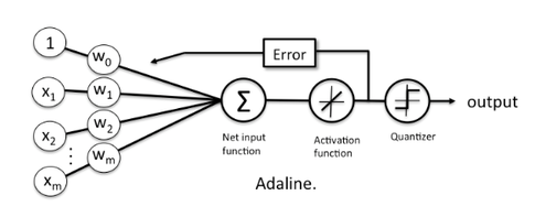
The key difference between Adaline and Perceptron is that the weights in Adaline are updated on a linear activation function rather than the unit step function as is the case with Perceptron.
In Adaline, the linear activation function is simply the identity function of the net input,
\(\phi(z) = z,\ \ where\ z = w^Tx\)
\(w\) being the weight vector and \(x\) being the sample (row from the feature matrix)
Minimizing the cost function
One of the main ideas of supervised machine learning algorithms is to optimize a defined objective function during the learning process. This is often the cost function we want to minimize. Observing or ploting this functino should give us a performance metric for how well the learning process went. Looking at this, we can further optimize other parameters if needed.
Coming back Adaline, this cost function is \(J\) is defined as the Sum of squared errors (SSE) between the calculated outcome by the activation function and the true class label
Note: Here the outcome is a real value (output by the activation function), not {1, -1} as in the case of Perceptron’s unit step function.
\(J(w) = \frac{1}{2}\sum_{i}{(y^{(i)} - \phi(z^{(i)}))}^2\)
\(y^{(i)}\) is the true class label
\(\phi(z^{(i)})\) is the net input form the activation function.
an error is defined as the difference between those two.
Advantages of this cost function
The advantages of choosing this continuous valued cost function are:
- It becomes differentiable
- It is convex shaped (we can use gradient descend)
We can use this simple yet powerful optimizing technique called gradient descend to find the weights that minimize our cost function. The concept is important enough to warrant its own blog post but i’ll try to summarize it in a few lines here for context.
Gradient descend can be thought of as climbing down a hill until a global or a local cost minimum is reached.
Using gradient descend, we can now update our weights each iteration following the rule:-
\(w := w + \Delta w\)
where, \(\Delta w = -\eta \nabla J(w)\)
where, \(\eta\) = Learning rate and \(\nabla J(w)\) is the gradient of J(w)
Important difference
One other important difference between Adaline and Perceptron is that in adaline, the weights are updated only once at the end of an iteration over the entire dataset, unlike the Perceptron, where the weights are updated after every single sample in every iterations