Introduction
Logistic Regression is one of the most widely used algorithms for classification in the industry today.
Inspite of the name, Logistic Regression, just like the previously discussed Adaline model is a linear model for binary classification and NOT regression. It just as-well can be extended to work as a multi-class classifier via using techniques like the OneVersesRest(OvR) technique.
The reasons for Logistic Regression’s popularity?
- It is an easy model to implement and understand
- Performs very well on linearly seprable data classes
Logistic Regression is a lot similar to Adaline model but, with a different activation and cost function, as we we’ll see.
New Terms and functions
Odds ratio
The odds in favor of a particular event, the odds ratio can be written as \(\frac{p}{(1-p)}\) where \(p\) is the probability of the positive event (positive = the event we are looking for, not necessarily in a good context, eg: presence of a disease)
logit function
\(logit(p) = log \frac{p}{(1-p)}\)
where again \(p\) is the probability of the positive event The logit function takes input values in the range 0 to 1 and transforms them to values over the entire real-number range, which we can use to express a linear realtionship between feature values and log-odds:
\[ logit(p(y=1|x)) = w_{1}x_{1} + w_{2}x_{2} + … + w_{m}x_{m} = \sum_{i=0}^{m} w_{i}x_{i} = w^Tx \] here, \(p(y=1 | x)\) is the conditional probability that a particular sample belongs to class 1 given features x.
Illustrative Diagram:-
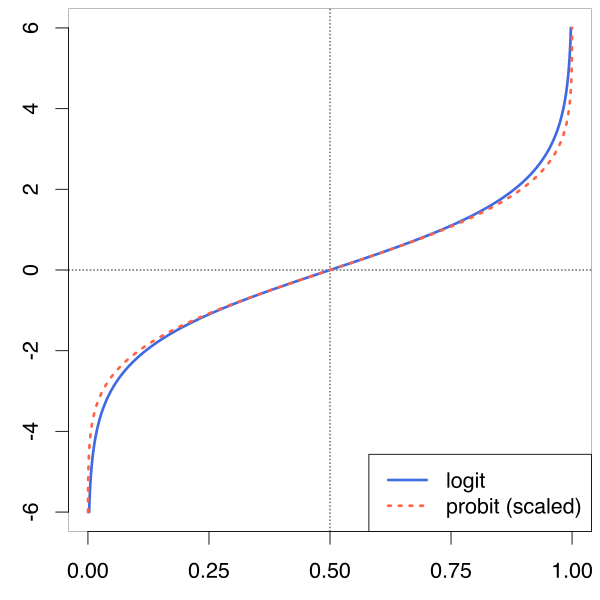
sigmoid function
we are actually interested in predicting the probability that a certain sample belongs to a class, which is the inverse form of logit function. It is called the logistic sigmoid, often abbreviated to simple sigmoid function because of its characteristic S-shape:
\(\phi(z) = \frac{1}{1+e^{-z}}\)
where \(z\) is the net input, ie the linear combination of the weights and sample features, \(z = w^Tx\)
Illustrative Diagram:-

we can see that \(\phi(z)\) approaches 1 if z goes to infinity \((z -> \infty)\) as \(e^{-z}\) becomes dismally small, and it reaches - 0 when z goes to -inifinity.
There’s an intercept at \(\phi(0) = 0.5\)
The Schematic
The following illustrates the difference between Adaline and Logistic Regression rules
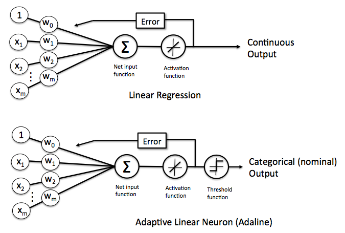
key differences
The activation function in Logistic Regression is a sigmoid function, instead of the linear identity function in Adaline.
The output from the Logistic Regression’s Activation function is the probability that the given sample belongs to class 1.
If we want the probability that the sample belongs to class 0, subtract the output from 1
The cost function is different
Logistic Regression has a final threshold function (not seen in the schematic) such that: If the probability of the sample is \(\geq\) 0.5, it is classified as class 1 If the probability of the sample is \(<\) 0.5, it is classifed as class 0
\(\hat y\) = 1 if \(\phi(z) \geq 0.5\), \(0\) otherwise.
Looking at the sigmoid function, this is equivalent to \(\hat y = 1\) if \(z\geq 0.0\), else \(0\) otherwise.
The cost function
Long story short, the cost function for logistic regression is:-
\[ J(w)\ =\ \sum_{i=1}^{n} \big[ -y^{(i)}log(\hat y) - (1-y^{(i)})log(1-\hat y)\big] \]
where:-
- \(y^{(i)}\) is the \(i_{th}\) class label in the target vector (a 1 or a 0)
- \(\hat y = \phi(z)\) i.e. the probability output by the activation function. \(\in [0, 1]\)
For better understanding, lets look at the cost calculation for a single sample training instance \[ J(\phi(z), y;w) = -ylog(\phi(z)) - (1-y)(log(1 - \phi(z))) \]
so, this means: -
- when y = 1, the term \((1 - y)\) in cost function becomes 0, thus leaving \(J(\phi(z), y;w) = -log(\phi(z))\)
- Now, as we want to Minimize our cost function, we want \(log(\phi(z))\) as big as possible such that when multiplied by \(-1\), it is as small as possible, Thus we want \(\phi(z)\) to be as large as possible.
Since, \(\phi(z)\) is a sigmoid function, thus the max value it can have is \(1\), which is as close to class 1 as possible. See how it all fits together?
- when y = 0, the term \(-ylog(\phi(z))\) in the cost function becomes 0, thus leaving \(J(\phi(z), y;w) = -(log(1 - \phi(z)))\)
Now, as we want to minimize our cost function, we want \(log(1 - \phi(z))\) to be as large as possible, such that when multiplied by -1, it becomes as small as possible. This only happens when \(\phi(z)\) is as small as possible, which is 0, since it is afterall, a sigmoid function.
Read through all that? Wow.
You now know quite a lot about the basis and theory of the Linear Regression Binary classification model : )