Introduction
Support Vector Machines (or SVMs) enjoy a really high popularity amongst machine learning practitioners, to the point of being ubiquitous, they are everywhere!
A Support Vector Machine or SVM is a supervised learning algorithm, which can really can be thought of as an extension of the Perceptron model.
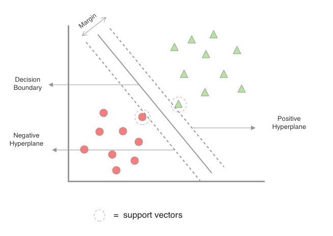
The big idea here is to maximize the decision margins, which is defined as the distance between the separating hyperplane (the decision boundary) and the training samples closest to the hyperplane on either side, which are the so called support vectors
When there are multiple hyperplanes that act as a decision boundary (see figure).

SVM algorithm says that we should chose the one with the maximum margin. They are sometimes referred as Maximum-Margin classifiers because of this characteristic.
The rationale behind having decision boundaries with large margins is that they tend to have a lower generalization error (better at predict outcome values for previously unseen data), whereas models with small margins are prone to overfitting .
The Mathematics of SVMs
if the decision-boundary is a hyperplane, which can be expressed as \(w_{0} + w^{T}x = 0\), where \(w\) is the weight vector, \(w_{0}\) the bias and \(x\) is the feature vector. Then the planes parallel to the hyperplanes, which we call the positive and negative hyperplanes can be expressed as:
- \(w_{0}+w^{T}x_{pos} = 1\) or simply \(\ \ w_{0} + w^{T}x_{pos} - 1 = 0\) \(\ \ \ \ \ \ \ \ \ (1)\)
And
- \(w_{0}+w^{T}x_{neg} = -1\) or simply \(\ \ w_{0} + w^{T}x_{neg} + 1 = 0\) \(\ \ \ \ \ \ (2)\)
If we subtract equations \((1)\) and \((2)\) from each other, we get:
\(\implies w^{T}(x_{pos} - x_{neg}) = 2\)
we can normalize this equation by the length of vector _w_m which is defined as:
\(\parallel w \parallel = \sqrt{\sum^{i}_{j=1} w^2_j}\)
we arrive at the following equation:
\(\dfrac {w^T(x_{pos} - x_{neg})} {\parallel w \parallel} = \dfrac {2}{\parallel w \parallel}\)
The left side of the preceding equation can be interpreted as the distance between the positive and negative hyperplane, which is the so-called margin that we want to maximize.
Now, the objective function of the SVM becomes the maximization of this margin by maximizing \(\dfrac {2}{\parallel w \parallel}\) under the constraint that the samples are classified correctly, which can be expressed as:
\(w_{0} + w^Tx^{(i)} \geq 1 \ \ if\ \ y^{(i)} = 1\)
\(w_{0} + w^Tx^{(i)} \leq -1 \ \ if\ \ y^{(i)} = -1\)
for i = 1 . . . N where, N is the number of samples in our dataset.
Those two equations are just a formal way of saying that all positive samples should fall ahead of the positive hyperplane and all the negative samples should fall behind the negative hyperplane. which can also more compactly be written as
\(y^{(i)}(w_0+w^Tx^i) \geq 1 \ \ \forall _i\)
In practice though, it is easier to Minimize the reciprocal term \(\dfrac {{\parallel w \parallel}^2} {2}\), which can be solved by quadratic programming, whose details are out of the scope of this post.
But what about non-linearity?
We already know from the post on Perceptron Algorithm, that it never converges on data which is not linearly separable. Does SVMs, with their linear decision boundaries also suffer from indefinite non-convergence ?
They would, if not for something called a Slack variable. The motivation for introducing the slack variable \(\xi\) was to relax the linear constraints for nonlinearly separable data to allow convergence in presence of misclassifications, under appropriate cost penalties.
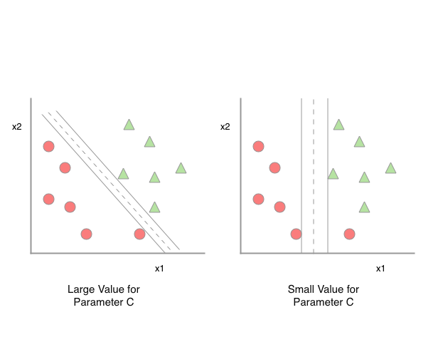
What ^ that means in plain English is you allow some misclassifications, given you agree to their penalty cost. If the penalty is low and misclassifying it does give you a better margin, then you misclassify it. If the penalty is high, you do not misclassify it at the cost of a reduced margin. (see figure)
The positive value slack variable is simply added to the linear constraints:
\(w_0 + w^Tx^{(i)} \geq 1 - \xi^{(i)} \ \ if\ \ y^{(i)} = 1\)
and
\(w_0 + w^Tx^{(i)} \geq -1 + \xi^{(i)} \ \ if\ \ y^{(i)} = -1\)
for \(i\) = 1 … N, where N is the number of samples in our dataset.
So, the new objective to be minimized (subject to constraints) becomes:
\(\dfrac 1 2 {\parallel w \parallel}^2 + C\Big(\sum_i \xi^{(i)}\Big)\)
Via, the variable \(C\), we can control the penalty for misclassification.
- Large values of \(C\) correspond to larger error penalty
- Smaller values of \(C\) indicate that we are less strict about misclassification errors.
Note:- The variable \(C\) became convention, you might see it at many places, just hanging around, many times without any context, for eg: in the Decision Trees Learning Algorithm, it is thus in general, a good idea to be familiar with it.
We can use the variable \(C\) to control the width of the margin, thus tuning the bias-variance trade-off as seen in the figure below.
The code
This is how you import a SVC classifier from sci-kit learn python module and feed it the training data for it to learn (fit) from.
from sklearn.svm import SVC

svm = SVC(kernel='linear', C=1.0, random_state=1)
svm.fit(X_train, y_train)
The parameter C is the same C we saw earlier
Summary
whew, That was a handful. Lets review what we learned in the post:
- We learned what Support Vector Machines are and what they do.
- We learned about the questions SVMs answer.
- We learned about the fundamental Mathematics behind SVMs.
- We learned about how SVMs handle non-linearity.
- We learned about how to control the cost penalty for misclassifications in case of nonlinearly separable data.
Conclusion
We learned that support vector machines are a really popular choice with ML practitioners, and for good reason. It is a really handy algorithm and to understand, simply because it can be found everywhere, from building classifiers to the example section of your favorite machine learning library. Apart from the ease of use, a major reason for SVM’s popularity is the Kernel Trick or the Kernel Method, which may be a topic for illustrations in a future post, stay tuned and keep learning.